這一章我們終於要討論到影像辨識的重頭戲啦!通常,處理影像類別我們會用Convolutional Neurel Network,聽起來很難很厲害,不過只要了解背後概念你就知道為什麼要這麼做了,讓我們看下去。
本單元程式碼可於Github下載。
影像有什麼特性
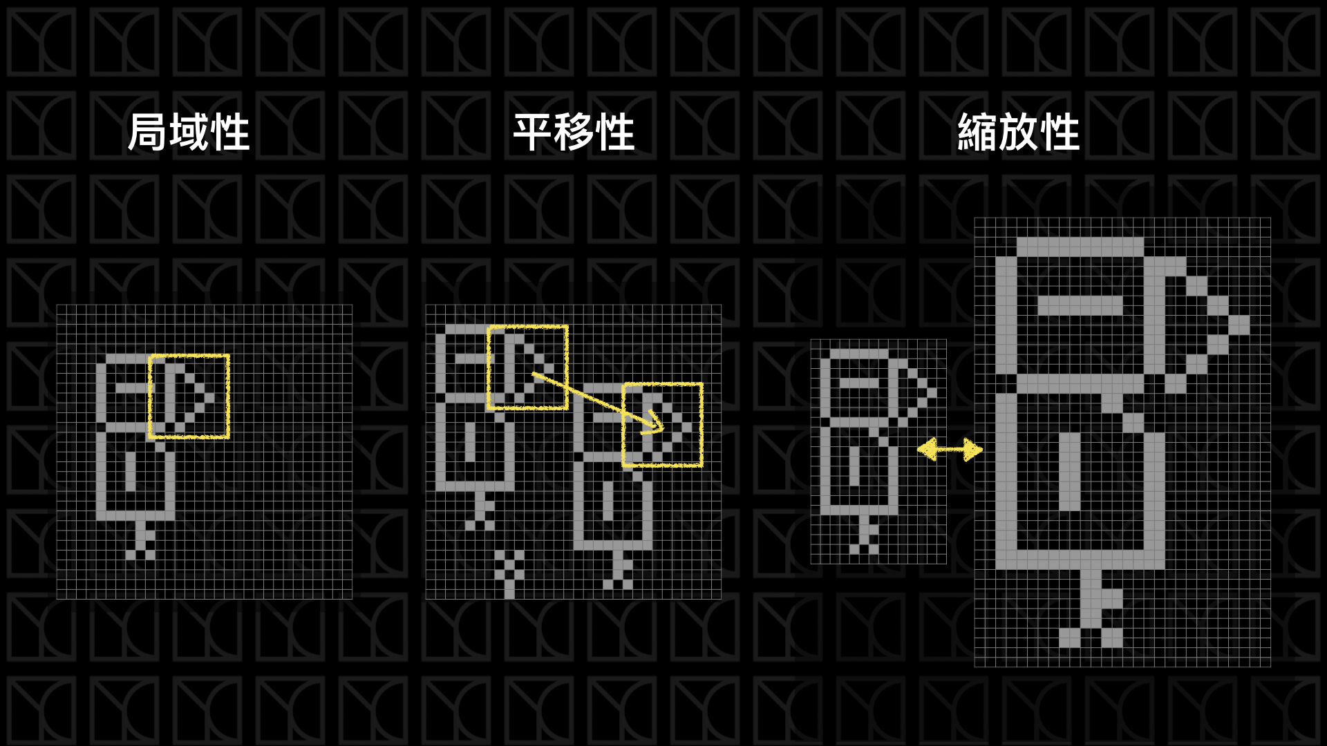
來想一下,影像具備了什麼特性?
(1) 局域性:通常物件只在一個局域的範圍裡有效,而與太遠的距離無關,譬如我要找一張圖的鳥嘴,鳥嘴的呈現在一張圖當中只會出現在一個小範圍內,所以其實只需要評估這小範圍就可以判斷這是不是鳥嘴了。
(2) 平移性:通常一張圖任意平移並不影響它的意義,一隻鳥不管是放在圖片的左上角還是右下角,牠都是一隻鳥。
(3) 縮放性:通常一張圖我把它等比例的放大縮小是不影響它的意義的。
DNN用在影像上的侷限
我們剛剛看過了影像具有的三種特性:「局域性」、「平移性」和「縮放性」,那我們就拿這三種特性來檢驗上一回的DNN Classification。
DNN有「局域性」嗎?沒有,因為我們把圖片攤平處理,原本應該是相鄰的關係就被打壞了,事實上DNN的結構會造成每個Input都會同時影響下一層的「每個」神經元,所以相不相鄰根本沒關係,因為每個Pixels的影響是全域的。
DNN有「平移性」嗎?沒有,沒有局域性就沒有平移性。
DNN有「縮放性」嗎?我們沒有一層試著去縮放,而且圖片已經被攤平了,難以做到縮放的效果。
所以其實使用DNN並不能好好的詮釋影像。
Convolutional Neurel Network (CNN)
我們需要引入新的架構來處理影像,讓它可以擁有以上三種特性,Convolutional Neurel Network (CNN)此時就登場了,CNN有兩大新要素:Convolution Layer和Pooling Layer,Convolution Layer為我們的Model添加了局域性和平移性,而Pooling Layer則讓Model擁有縮放的特性。
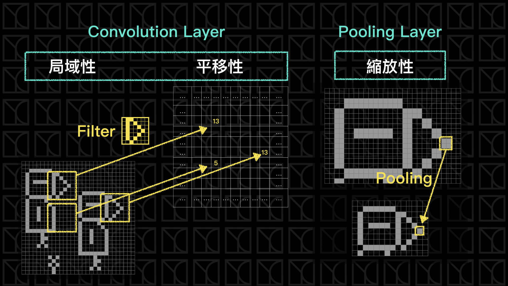
Convolution Layer是由Filters所構成的,Filters可以想像是一張小圖,以上面的例子,Filter是一個鳥嘴的小圖,這張小圖要怎麼去過濾原圖呢?答案是使用Convolution(卷積),把小圖疊到大圖的任意位置,接下來將大圖小圖對到的相應元素相乘起來再加總一起,然後在另外一張表格中填入這個加總值,接下來移動Filter,重複的動作再做一次,如此循環並將值陸續填入表格中,這表格最後就會像是另外一張圖一樣,而這張圖可以繼續串另外的Neurel Network,這就是Convolution Layer的計算方法。
舉個例子,假設我今天有矩陣A:
[[1, 2, 3, 4],
[4, 5, 6, 7],
[7, 8, 9,10],
[1, 3, 5, 7]]
然後再有一個Filter:
[[1, 0, 0],
[0, 1, 0],
[0, 0, 0]]
使用Filter對A做Convolution得到B為:
[[6, 8 ],
[12,14]]
原本4x4的矩陣做了Convolution後變成了2x2的矩陣,原因在於邊界限制了Filter的移動,那如果我想要讓Convolution玩的矩陣維持在4x4,怎麼做?我們可以在邊緣的地方鋪上0就可以達到這樣的效果,來試試看,先將矩陣A擴張成矩陣C:
[[0, 0, 0, 0, 0, 0],
[0, 1, 2, 3, 4, 0],
[0, 4, 5, 6, 7, 0],
[0, 7, 8, 9,10, 0],
[0, 1, 3, 5, 7, 0],
[0, 0, 0, 0, 0, 0]]
再使用Filter對C做Convolution會得到D為:
[[1, 2, 3, 4],
[4, 6, 8,10],
[7,12,14,16],
[1,10,13,16]]
而此時D就是一個4x4的矩陣。
Convolution的過程造成怎麼樣的效果呢?當Filter是一個鳥嘴的小圖,一旦遇到與鳥嘴相似的局部,此時加總的值會是一個大的值,如果是一個和鳥嘴無關的局部此時的值會是一個小的值,所以這個Filter具有將特定特徵篩選出來的能力,符合特徵分數高不符合則分數低,因此局部的特徵變得是有意義的,此時我的Model就具有局域性,而且藉由Filter的平移掃視,這個特徵就具有可平移的特性。
Convolution Layer不同於Fully-connected Layer有兩點,第一,每個Pixels間有相對的距離關係,擁有上下左右的關係才有辦法構成一張圖,第二,除了有距離上的關係以外,它還能在有限範圍內抓出一種特徵模式,所以我們將可以使用影像的語言來做特徵轉換和抓取特徵。
實際情況下,Filter上的Weights是會自行調整的,Model Fitting的時候,Model會根據數據自行訓練出Filter,也就是說機器可以自行學習出圖片的特徵。通常這樣的Filters會有好幾個,讓機器可以有更多維度可以學習。
接下來來看Pooling Layer如何讓Model擁有檢視縮放的特性?
先來看在影像上如何做到放大縮小,以Pixels的觀點來看,最簡單的放大方法是,在每個既有的Pixels附近增加一些與它們相似的新Pixel,這樣做就像是將原本的小圖直接拉成大圖,畫質雖然很差,不過這是最簡單的放大方法。那麼縮小就相反操作,把一群附近的Pixels濃縮成一個Pixel當作代表,就可以達到縮小圖片的效果。
所以回到Pooling Layer的討論,Pooling做的事情就是在縮小圖片,例如我使用2x2來做Pooling,它會在原圖上以2x2來掃描,所以會有四個元素被檢視,然後從這四個值當中產生一個代表值,把原本2x2的Pixels減少成這個1x1的代表值,如果是Max Pooling就是從四個中選最大的那個,如果是Average Pooling則是平均四個值得到平均值,通常如果是2x2的Pooling我們會以每2格一跳的方式掃視,如果是3x3則會以每3格一跳,以此類推。
Convolution Layer
來看一下Tensorflow如何實作Convolution Layer。
| import random
import numpy as np
import tensorflow as tf
import matplotlib.pyplot as plt
tf.logging.set_verbosity(tf.logging.ERROR)
# Config the matplotlib backend as plotting inline in IPython
%matplotlib inline
|
 1
 2
 3
 4
 5
 6
 7
 8
 9
10
11
12
13
14
15
16
17
18
19
20
21
22
23
24
25 | with tf.Session() as sess:
img =tf.constant([[[[1], [2], [0], [0], [0]],
[[3], [0], [0], [1], [2]],
[[0], [0], [0], [3], [0]],
[[1], [0], [0], [1], [0]],
[[0], [0], [0], [0], [0]]]], tf.float32)
# shape of img: [batch, in_height, in_width, in_channels]
filter_ = tf.constant([[[[1]], [[2]]],
[[[3]], [[0]]]], tf.float32)
# shape of filter: [filter_height, filter_width, in_channels, out_channels]
conv_strides = (1,1)
padding_method = 'VALID'
conv = tf.nn.conv2d(
img,
filter_,
strides=[1, conv_strides[0], conv_strides[1], 1],
padding=padding_method
)
print('Shape of conv:')
print(conv.eval().shape)
print('Conv:')
print(conv.eval())
|
1
2
3
4
5
6
7
8
9
10
11
12
13
14
15
16
17
18
19
20
21
22 | Shape of conv:
(1, 4, 4, 1)
Conv:
[[[[14.]
[ 2.]
[ 0.]
[ 3.]]
[[ 3.]
[ 0.]
[ 2.]
[14.]]
[[ 3.]
[ 0.]
[ 6.]
[ 6.]]
[[ 1.]
[ 0.]
[ 2.]
[ 1.]]]]
|
首先一開始是圖片img的部分,Rank為4,每個維度分別為[batch, in_height, in_width, in_channels],in_channels的部分一般是RGB,這邊我採用和MNIST相同的灰階表示,所以in_channels只有1個維度。
filter_的部分Rank為4,每個維度分別為[filter_height, filter_width, in_channels, out_channels],當如果我想要使用多個filters的時候,我的out_channels就不只1而已,如果有RGB的話,in_channels則會是3。
接下來來看一下tf.nn.conv2d裡頭的參數strides,這可能會讓人感到困惑,它的設定值是[1, conv_strides[0], conv_strides[1], 1],我特別把第二、三項額外用conv_strides來表示,因為這兩個值才是真正代表在圖片上平移每步的距離,那第一項和最後一項的1代表什麼意義呢?是這樣的,Tensorflow是站在維度的角度看平移這件事情,這四個維度分別表示[batch, in_height, in_width, in_channels]的移動量,所以一般情況下只有in_height和in_width需要指定平移的距離。
最後一個參數就是padding,有兩種可以選擇,分別為VALID和SAME,VALID指的就是沒有額外鋪上0的邊界的情形,SAME則是額外鋪上0的邊界,並且使得輸出的維度和輸入一樣。
Pooling Layer
接下來來看Tensorflow如何實作Pooling Layer。
1
2
3
4
5
6
7
8
9
10
11
12 | with tf.Session() as sess:
img =tf.constant([[[[1], [2], [0], [0]],
[[3], [0], [0], [1]],
[[0], [0], [0], [3]],
[[1], [0], [0], [1]]]], tf.float32)
# shape of img: [batch, in_height, in_width, in_channels]
pooling = tf.nn.max_pool(img, ksize=[1, 2, 2, 1], strides=[1, 2, 2, 1], padding='VALID')
print('Shape of pooling:')
print(pooling.eval().shape)
print('Pooling:')
print(pooling.eval())
|
| Shape of pooling:
(1, 2, 2, 1)
Pooling:
[[[[3.]
[1.]]
[[1.]
[3.]]]]
|
tf.nn.max_pool的參數中ksize代表kernel size,也就是要Pooling的大小,一樣依照Input layer的Rank去配置,還有strides決定平移的方法。
最簡單的CNN架構:LeNet5
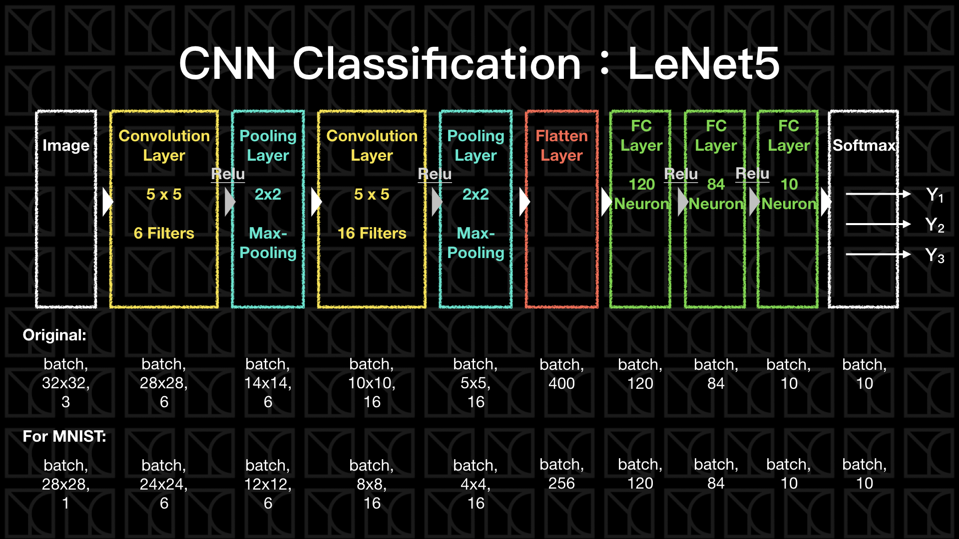
接下來我們就真正的來實作一下CNN網路,和之前兩個單元一樣,我們拿MNIST的分類問題來當作題目。
本單元介紹的是最簡單的CNN Classification的方法—LeNet5,流程如上圖所示。
(1) conv1+relu+pooling2:一開始使用Convolution抓取圖片中的特徵,並且加入Activation Function使得Model具有非線性因子,通常在這種非常深的網路,我們會採用Relu,它的好處是不會出現「梯度消失」(Vanishing Gradient)的問題,如果你使用像是tanh或sigmoid這類在飽和區梯度接近0的函數,則就很有可能在深網路的情形下,造成一開始的幾個Layers梯度太小的問題,也就是前面幾層我們無法訓練到,而Relu在Turn-on的情況下是線性的,不會有飽和的問題,也就不會出現「梯度消失」。做完Convolution後,我們已經對於這個圖片有一點認識了,所以減少一些Pixels來減少一些計算量,所以加入Pooling Layer,注意喔!Pooling Layer結束之後,不需要再做一次Activation,因為Pooling只是用來平均前面的結果而已。
(2) conv3+relu+pooling4:做第二次的圖片特徵抽取。
(3) fatten5:將抽取完的特徵完全打平,為了接下來的Fully-connected Network做準備。
(4) fc6+fc7+fc8+softmax:這個部分就和之前DNN Classification做的事情一樣,全盤考慮每一個擷取來的特徵,並且非線性的轉換成最後可以分為相應的10種類別。
接下來我們看一下程式碼要怎麼寫?
 1
 2
 3
 4
 5
 6
 7
 8
 9
10
11
12
13
14
15
16
17
18
19
20
21
22
23
24
25
26
27
28
29
30
31
32
33
34
35
36
37
38
39
40
41
42
43
44
45
46
47
48
49
50
51
52
53
54
55
56
57
58
59
60
61
62
63
64
65
66
67
68
69
70
71
72
73
74
75
76
77
78
79
80
81
82
83
84
85
86
87
88
89
90
91
92
93
94
95
96
97
98
99
100
101
102
103
104
105
106
107
108
109
110
111
112
113
114
115
116
117
118
119
120
121
122
123
124
125
126
127
128
129
130
131
132
133
134
135
136
137
138
139
140
141
142
143
144
145
146
147
148
149
150
151
152
153
154
155
156
157
158
159
160
161
162
163
164
165
166
167
168
169
170
171
172
173
174
175
176
177
178
179
180
181
182
183
184
185
186
187
188
189
190
191
192
193
194
195
196
197
198
199
200
201
202
203
204
205
206
207
208
209 | class CNNLogisticClassification:
def __init__(self, shape_picture, n_labels,
learning_rate=0.5, dropout_ratio=0.5, alpha=0.0):
self.shape_picture = shape_picture
self.n_labels = n_labels
self.weights = None
self.biases = None
self.graph = tf.Graph() # initialize new grap
self.build(learning_rate, dropout_ratio, alpha) # building graph
self.sess = tf.Session(graph=self.graph) # create session by the graph
def build(self, learning_rate, dropout_ratio, alpha):
with self.graph.as_default():
### Input
self.train_pictures = tf.placeholder(tf.float32,
shape=[None]+self.shape_picture)
self.train_labels = tf.placeholder(tf.int32,
shape=(None, self.n_labels))
### Optimalization
# build neurel network structure and get their predictions and loss
self.y_, self.original_loss = self.structure(pictures=self.train_pictures,
labels=self.train_labels,
dropout_ratio=dropout_ratio,
train=True, )
# regularization loss
self.regularization = \
tf.reduce_sum([tf.nn.l2_loss(w) for w in self.weights.values()]) \
/ tf.reduce_sum([tf.size(w, out_type=tf.float32) for w in self.weights.values()])
# total loss
self.loss = self.original_loss + alpha * self.regularization
# define training operation
optimizer = tf.train.GradientDescentOptimizer(learning_rate)
self.train_op = optimizer.minimize(self.loss)
### Prediction
self.new_pictures = tf.placeholder(tf.float32,
shape=[None]+self.shape_picture)
self.new_labels = tf.placeholder(tf.int32,
shape=(None, self.n_labels))
self.new_y_, self.new_original_loss = self.structure(pictures=self.new_pictures,
labels=self.new_labels)
self.new_loss = self.new_original_loss + alpha * self.regularization
### Initialization
self.init_op = tf.global_variables_initializer()
def structure(self, pictures, labels, dropout_ratio=None, train=False):
### Variable
## LeNet5 Architecture(http://yann.lecun.com/exdb/lenet/)
# input:(batch,28,28,1) => conv1[5x5,6] => (batch,24,24,6)
# pool2 => (batch,12,12,6) => conv2[5x5,16] => (batch,8,8,16)
# pool4 => fatten5 => (batch,4x4x16) => fc6 => (batch,120)
# (batch,120) => fc7 => (batch,84)
# (batch,84) => fc8 => (batch,10) => softmax
if (not self.weights) and (not self.biases):
self.weights = {
'conv1': tf.Variable(tf.truncated_normal(shape=(5, 5, 1, 6),
stddev=0.1)),
'conv3': tf.Variable(tf.truncated_normal(shape=(5, 5, 6, 16),
stddev=0.1)),
'fc6': tf.Variable(tf.truncated_normal(shape=(4*4*16, 120),
stddev=0.1)),
'fc7': tf.Variable(tf.truncated_normal(shape=(120, 84),
stddev=0.1)),
'fc8': tf.Variable(tf.truncated_normal(shape=(84, self.n_labels),
stddev=0.1)),
}
self.biases = {
'conv1': tf.Variable(tf.zeros(shape=(6))),
'conv3': tf.Variable(tf.zeros(shape=(16))),
'fc6': tf.Variable(tf.zeros(shape=(120))),
'fc7': tf.Variable(tf.zeros(shape=(84))),
'fc8': tf.Variable(tf.zeros(shape=(self.n_labels))),
}
### Structure
conv1 = self.get_conv_2d_layer(pictures,
self.weights['conv1'], self.biases['conv1'],
activation=tf.nn.relu)
pool2 = tf.nn.max_pool(conv1,
ksize=[1, 2, 2, 1], strides=[1, 2, 2, 1], padding='VALID')
conv3 = self.get_conv_2d_layer(pool2,
self.weights['conv3'], self.biases['conv3'],
activation=tf.nn.relu)
pool4 = tf.nn.max_pool(conv3,
ksize=[1, 2, 2, 1], strides=[1, 2, 2, 1], padding='VALID')
fatten5 = self.get_flatten_layer(pool4)
if train:
fatten5 = tf.nn.dropout(fatten5, keep_prob=1-dropout_ratio[0])
fc6 = self.get_dense_layer(fatten5,
self.weights['fc6'], self.biases['fc6'],
activation=tf.nn.relu)
if train:
fc6 = tf.nn.dropout(fc6, keep_prob=1-dropout_ratio[1])
fc7 = self.get_dense_layer(fc6,
self.weights['fc7'], self.biases['fc7'],
activation=tf.nn.relu)
logits = self.get_dense_layer(fc7, self.weights['fc8'], self.biases['fc8'])
y_ = tf.nn.softmax(logits)
loss = tf.reduce_mean(
tf.nn.softmax_cross_entropy_with_logits(labels=labels,
logits=logits))
return (y_, loss)
def get_dense_layer(self, input_layer, weight, bias, activation=None):
x = tf.add(tf.matmul(input_layer, weight), bias)
if activation:
x = activation(x)
return x
def get_conv_2d_layer(self, input_layer,
weight, bias,
strides=(1, 1), padding='VALID', activation=None):
x = tf.add(
tf.nn.conv2d(input_layer,
weight,
[1, strides[0], strides[1], 1],
padding=padding), bias)
if activation:
x = activation(x)
return x
def get_flatten_layer(self, input_layer):
shape = input_layer.get_shape().as_list()
n = 1
for s in shape[1:]:
n *= s
x = tf.reshape(input_layer, [-1, n])
return x
def fit(self, X, y, epochs=10,
validation_data=None, test_data=None, batch_size=None):
X = self._check_array(X)
y = self._check_array(y)
N = X.shape[0]
random.seed(9000)
if not batch_size:
batch_size = N
self.sess.run(self.init_op)
for epoch in range(epochs):
print('Epoch %2d/%2d: ' % (epoch+1, epochs))
# mini-batch gradient descent
index = [i for i in range(N)]
random.shuffle(index)
while len(index) > 0:
index_size = len(index)
batch_index = [index.pop() for _ in range(min(batch_size, index_size))]
feed_dict = {
self.train_pictures: X[batch_index, :],
self.train_labels: y[batch_index],
}
_, loss = self.sess.run([self.train_op, self.loss],
feed_dict=feed_dict)
print('[%d/%d] loss = %.4f ' % (N-len(index), N, loss), end='\r')
# evaluate at the end of this epoch
y_ = self.predict(X)
train_loss = self.evaluate(X, y)
train_acc = self.accuracy(y_, y)
msg = '[%d/%d] loss = %8.4f, acc = %3.2f%%' % (N, N, train_loss, train_acc*100)
if validation_data:
val_loss = self.evaluate(validation_data[0], validation_data[1])
val_acc = self.accuracy(self.predict(validation_data[0]), validation_data[1])
msg += ', val_loss = %8.4f, val_acc = %3.2f%%' % (val_loss, val_acc*100)
print(msg)
if test_data:
test_acc = self.accuracy(self.predict(test_data[0]), test_data[1])
print('test_acc = %3.2f%%' % (test_acc*100))
def accuracy(self, predictions, labels):
return (np.sum(np.argmax(predictions, 1) == np.argmax(labels, 1))/predictions.shape[0])
def predict(self, X):
X = self._check_array(X)
return self.sess.run(self.new_y_, feed_dict={self.new_pictures: X})
def evaluate(self, X, y):
X = self._check_array(X)
y = self._check_array(y)
return self.sess.run(self.new_loss, feed_dict={self.new_pictures: X,
self.new_labels: y})
def _check_array(self, ndarray):
ndarray = np.array(ndarray)
if len(ndarray.shape) == 1:
ndarray = np.reshape(ndarray, (1, ndarray.shape[0]))
return ndarray
|
| from tensorflow.examples.tutorials.mnist import input_data
mnist = input_data.read_data_sets('MNIST_data/', one_hot=True)
train_data = mnist.train
valid_data = mnist.validation
test_data = mnist.test
|
| Successfully downloaded train-images-idx3-ubyte.gz 9912422 bytes.
Extracting MNIST_data/train-images-idx3-ubyte.gz
Successfully downloaded train-labels-idx1-ubyte.gz 28881 bytes.
Extracting MNIST_data/train-labels-idx1-ubyte.gz
Successfully downloaded t10k-images-idx3-ubyte.gz 1648877 bytes.
Extracting MNIST_data/t10k-images-idx3-ubyte.gz
Successfully downloaded t10k-labels-idx1-ubyte.gz 4542 bytes.
Extracting MNIST_data/t10k-labels-idx1-ubyte.gz
|
1
2
3
4
5
6
7
8
9
10
11
12
13
14
15
16
17
18
19
20 | model = CNNLogisticClassification(
shape_picture=[28, 28, 1],
n_labels=10,
learning_rate=0.07,
dropout_ratio=[0.2, 0.1],
alpha=0.1,
)
train_img = np.reshape(train_data.images, [-1, 28, 28, 1])
valid_img = np.reshape(valid_data.images, [-1, 28, 28, 1])
test_img = np.reshape(test_data.images, [-1, 28, 28, 1])
model.fit(
X=train_img,
y=train_data.labels,
epochs=10,
validation_data=(valid_img, valid_data.labels),
test_data=(test_img, test_data.labels),
batch_size=32,
)
|
1
2
3
4
5
6
7
8
9
10
11
12
13
14
15
16
17
18
19
20
21 | Epoch 1/10:
[55000/55000] loss = 0.0894, acc = 97.21%, val_loss = 0.0872, val_acc = 97.34%
Epoch 2/10:
[55000/55000] loss = 0.0532, acc = 98.41%, val_loss = 0.0589, val_acc = 98.30%
Epoch 3/10:
[55000/55000] loss = 0.0567, acc = 98.27%, val_loss = 0.0578, val_acc = 98.18%
Epoch 4/10:
[55000/55000] loss = 0.0384, acc = 98.85%, val_loss = 0.0475, val_acc = 98.56%
Epoch 5/10:
[55000/55000] loss = 0.0307, acc = 99.10%, val_loss = 0.0431, val_acc = 98.82%
Epoch 6/10:
[55000/55000] loss = 0.0299, acc = 99.09%, val_loss = 0.0388, val_acc = 98.88%
Epoch 7/10:
[55000/55000] loss = 0.0280, acc = 99.17%, val_loss = 0.0403, val_acc = 98.86%
Epoch 8/10:
[55000/55000] loss = 0.0233, acc = 99.31%, val_loss = 0.0372, val_acc = 99.02%
Epoch 9/10:
[55000/55000] loss = 0.0225, acc = 99.32%, val_loss = 0.0356, val_acc = 99.02%
Epoch 10/10:
[55000/55000] loss = 0.0234, acc = 99.27%, val_loss = 0.0411, val_acc = 98.84%
test_acc = 98.89%
|
太棒了!我們的預測效果如果跟之前的結果比較,在Epoch=3已經達到98.5%了,在Epoch=10更是高達99%!
圖像化
有這麼好的成果,我們不妨就拉進去看,裡面每個Filters究竟是長什麼樣子的?
先來看第一層Convolution的Filters。
| fig, axis = plt.subplots(1, 6, figsize=(7, 0.9))
for i in range(0,6):
img = model.sess.run(model.weights['conv1'])[:, :, :, i]
img = np.reshape(img, (5,5))
axis[i].imshow(img, cmap='gray')
plt.show()
|

再來看第二層Convolution的Filters。
| fig, axis = plt.subplots(12, 8, figsize=(10, 12))
for i in range(6):
for j in range(16):
img = model.sess.run(model.weights['conv3'])[:, :, i, j]
img = np.reshape(img, (5, 5))
axis[i*2+j//8][j%8].imshow(img, cmap='gray')
plt.show()
|

單看這些Filters似乎很難看出什麼?
我們試著丟幾張圖進去做Convolution,看一下在Filters的拆解之下圖片會變怎樣?
以下圖片的第一行表示原圖片,第二行表示做完第一次Convolution後的結果,第三行表示做完第二次Convolution後的結果。
 1
 2
 3
 4
 5
 6
 7
 8
 9
10
11
12
13
14
15
16
17
18
19
20
21
22
23
24
25
26 | fig, axis = plt.subplots(3, 16, figsize=(16, 3))
picture = np.reshape(test_img[0, :, :, :],(1, 28, 28, 1))
with model.sess.as_default():
conv1 = model.getConv2DLayer(picture,
model.weights['conv1'], model.biases['conv1'],
activation=tf.nn.relu)
pool2 = tf.nn.max_pool(conv1,
ksize=[1,2,2,1], strides=[1,2,2,1], padding='VALID')
conv3 = model.getConv2DLayer(pool2,
model.weights['conv3'], model.biases['conv3'],
activation=tf.nn.relu)
eval_conv1 = conv1.eval()
eval_conv3 = conv3.eval()
axis[0][0].imshow(np.reshape(picture, (28, 28)), cmap='gray')
for i in range(6):
img = eval_conv1[:, :, :, i]
img = np.reshape(img, (24, 24))
axis[1][i].imshow(img, cmap='gray')
for i in range(16):
img = eval_conv3[:, :, :, i]
img = np.reshape(img, (8, 8))
axis[2][i].imshow(img, cmap='gray')
plt.show()
|

 1
 2
 3
 4
 5
 6
 7
 8
 9
10
11
12
13
14
15
16
17
18
19
20
21
22
23
24
25
26 | fig, axis = plt.subplots(3, 16, figsize=(16, 3))
picture = np.reshape(test_img[10, :, :, :],(1, 28, 28, 1))
with model.sess.as_default():
conv1 = model.getConv2DLayer(picture,
model.weights['conv1'], model.biases['conv1'],
activation=tf.nn.relu)
pool2 = tf.nn.max_pool(conv1,
ksize=[1,2,2,1], strides=[1,2,2,1], padding='VALID')
conv3 = model.getConv2DLayer(pool2,
model.weights['conv3'], model.biases['conv3'],
activation=tf.nn.relu)
eval_conv1 = conv1.eval()
eval_conv3 = conv3.eval()
axis[0][0].imshow(np.reshape(picture, (28, 28)), cmap='gray')
for i in range(6):
img = eval_conv1[:, :, :, i]
img = np.reshape(img, (24, 24))
axis[1][i].imshow(img, cmap='gray')
for i in range(16):
img = eval_conv3[:, :, :, i]
img = np.reshape(img, (8, 8))
axis[2][i].imshow(img, cmap='gray')
plt.show()
|

1
2
3
4
5
6
7
8
9
10
11
12
13
14
15
16
17
18
19
20
21
22
23
24
25
26 | fig, axis = plt.subplots(3, 16, figsize=(16, 3))
picture = np.reshape(test_img[15, :, :, :], (1, 28, 28, 1))
with model.sess.as_default():
conv1 = model.getConv2DLayer(picture,
model.weights['conv1'], model.biases['conv1'],
activation=tf.nn.relu)
pool2 = tf.nn.max_pool(conv1,
ksize=[1,2,2,1], strides=[1,2,2,1], padding='VALID')
conv3 = model.getConv2DLayer(pool2,
model.weights['conv3'], model.biases['conv3'],
activation=tf.nn.relu)
eval_conv1 = conv1.eval()
eval_conv3 = conv3.eval()
axis[0][0].imshow(np.reshape(picture, (28, 28)), cmap='gray')
for i in range(6):
img = eval_conv1[:, :, :, i]
img = np.reshape(img, (24, 24))
axis[1][i].imshow(img, cmap='gray')
for i in range(16):
img = eval_conv3[:, :, :, i]
img = np.reshape(img, (8, 8))
axis[2][i].imshow(img, cmap='gray')
plt.show()
|

有看出什麼規律嗎?哈哈。